Introduction to Vision Transformers
Uncover how computers understand and interpret images
Computer vision is a field of artificial intelligence that enables computers to interpret and understand visual information from the world around them. This field has been dominated by convolutional neural networks (CNNs) for many years, as they have consistently achieved state-of-the-art results on tasks like image classification, object detection, and more. However, a new class of models based on the transformer architecture, originally developed for natural language processing (NLP), has recently made significant advancements in the computer vision domain. These models, known as Vision Transformers (ViTs), are reshaping the world of machine learning and AI.
This article explores an introduction to Vision Transformers, how they function, and highlights some of the state-of-the-art (SOTA) models that are defining this exciting frontier. This will prepare you with everything you need ready for our next article on fine-tuning vision transformers.
Before diving in, if you need help, guidance, or want to ask questions, join our Community and a member of the Marqo team will be there to help.
1. A Brief History of Transformers
As discussed in our previous article, transformers were introduced in 2017 in the infamous paper, ‘Attention is all You Need’ [1]. This paper changed the entire landscape of Natural Language Processing all thanks to one feature: the attention mechanism. In this context, attention allows us to embed contextual meaning into the word-token embeddings within a model.
Take any sentence for example, attention allows you to identify the relationship between related words in that sentence. The process starts with tokens being embedded into a vector space. With each embedding, we can compute similarity measures between other embeddings to see which words should be placed close together within the vector space. Take the example of fruits in the Figure below.

For further information on the attention mechanism and its role in transformers, visit our previous article here.
In Vision transformers, the transformer encoder is comprised of alternating layers of multi-head self-attention and feed-forward neural networks. The self-attention mechanism enables the model to weigh the importance of all other patches when encoding a particular patch, allowing it to capture both local features and global contextual information without being restricted by the receptive fields typical in CNNs.
Let’s take a look at this in more detail.
2. How do Vision Transformers Work?
The operations of a vision transformer can be broken down into several steps, each of which is crucial in its overall function.
Generating Image-Patch Embeddings
There are four main steps to generating image/patch embeddings:
- Split an image into image patches.
- Process those patches through a linear projection layer to get our initial patch embeddings.
- We pre-append a class embedding to those patch embeddings.
- Sum patch embeddings and positional embeddings.
Each of these steps can be seen in the Figure below.
.png)
Let’s discuss these steps in a little bit more detail.
1. Transformation of our Image to Image Patches
Recall in Natural Language Processing, we take a sentence and translate it into a list of tokens. We can do something similar but for images; breaking an image into image patches.

We could break the image into each of its pixels but then the issue of computation with attention arises. In attention, you’re comparing every item against every other item within your input sequence. If your input sequence is a relatively large image and you’re comparing pixels to pixels, the number of comparisons that you need to do becomes very very large, very quickly. To overcome this we create image patches. Once we’ve built these image patches, we move onto the linear projection step.
2. Linear Projection Step
We now use a linear projection layer. The purpose of this is to map our image patch arrays to image patch vectors.
.png)
By mapping these patches to patch embeddings, we’re reformatting them into the correct dimensionality to be input into our vision transformer. But… we’re not putting these into the vision transformer just yet.
3. Learnable Class Embedding
The next crucial step is the use of a Learnable Class Embedding. A special learnable embedding known as the class embedding or [CLS] token, is pre-appended to this sequence as seen in the Figure below. This CLS token is also present in BERT but it’s more crucial to the performance of Vision Transformers.

This extra class embedding interacts with the patch embeddings through the self-attention mechanism of transformer layers, allowing it to gather and integrate information from the entire image. After processing, the class embedding, which now contains a global representation of the image, is used for the final classification task. This method simplifies the design and enhances the model's ability to aggregate and utilize global image information effectively.
4. Adding Positional Embeddings
The final step before our patch embeddings can be passed into the transformer encoder lies with what are known as positional embeddings. These are very common in transformers as transformers themselves do not inherently have anything to track the position of inputs; there’s no order that is being considered. You might not realise it but this is very difficult when it comes to both language and vision. The order of words in a sentence and the position of image patches in an image are incredibly important.
The order of our image patches is important. Positional embeddings help the model differentiate between the different positions in the image and therefore, capture spatial relationships. These are learned embeddings that are added to the incoming patch embeddings before they are inputted into the transformer encoder.

After adding all of these, we have our final patch embeddings which are fed into our vision transformer that are processed through encoder layers. Let’s take a look at how this works!
Transformer Encoder
We’ve looked at generating image patch embeddings which is a crucial step before passing any information into the encoder layers. The core of the Vision Transformer consists of multiple encoder layers. These are comprised of two primary sub-layers: multi-head self-attention and feedforward neural networks. Let’s look at both of these in detail.
Multi-Head Self-Attention: This mechanism captures the relationships between different patches in the input sequence. For every patch embedding, the self-attention mechanism computes a weighted sum of all the patch embeddings where the weights are determined by the relevance of each patch to the current one. Thus, the model is able to focus on important patches while also considering the local and global context. Instead of using a single attention head, multiple heads are used to capture different aspects of the relationships in parallel. The outputs of these heads are concatenated and linearly transformed.
Feedforward Neural Networks: Subsequently, the FFNs, consisting of fully connected layers and activation functions, further process these representations. Through a series of transformations and non-linear activations, the FFNs enhance the features extracted by the self-attention mechanism, enabling the model to learn complex relationships and patterns within the image. Essentially, refining and enriching the representations of image patches, ultimately contributing to the model's ability to understand and classify images effectively.
Prediction Head
After the image patches have been processed by the transformer encoder, the resulting representations need to be further processed to make predictions for specific tasks, such as image classification or object detection. The MLP head, or Multilayer Perceptron head, is a set of fully connected layers that perform this task-specific processing. It takes the output from the transformer encoder and applies additional transformations to prepare the data for the final classification or detection step.
The overall infrastructure of a Vision Transformer and its transformer encoder can be seen below.
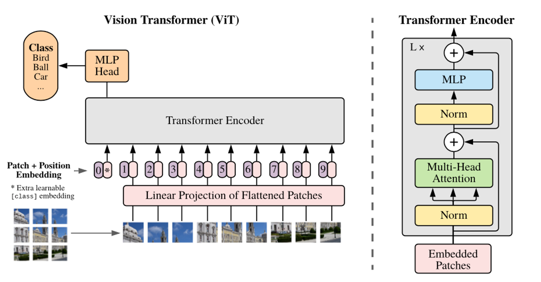
Awesome!
3. Conclusion
In this article, we’ve explored the architecture behind Vision Transformers. From taking an input image, creating embedded patches to the transformer encoder, we’ve uncovered a range of crucial steps involved in this architecture. Join us in the next article to put everything we’ve learned into action by training and fine-tuning vision transformers through code!
4. References
[1] A. Vaswani, et al. Attention is All You Need (2017)
[2] A. Dosovitskiy et al. An Image is Worth 16x16 Words: Transformers for Image Recognition at Scale (2020)