Train and Fine-Tune Sentence Transformer Models

Next Module →

← Back to Course Menu

Sections

As we saw in the previous article, sentence embeddings have significantly evolved since the introduction of BERT, with SBERT marking a major advancement in this field. BERT introduced deep contextualized embeddings but was inefficient for comparing sentence pairs. SBERT improved on this by producing fixed-sized sentence embeddings, enhancing performance for tasks like semantic similarity. Since the SBERT paper, many more sentence transformer models have been built, offering more accurate and efficient sentence embeddings by leveraging improved training and fine-tuning techniques.

But what exactly is training and fine-tuning? Training refers to the initial phase where a model learns patterns and representations from scratch using a large dataset, adjusting its parameters to minimize error through iterative optimization techniques. This foundational training provides the model with a broad understanding of general features and relationships within the data. Fine-tuning, on the other hand, is a subsequent, more focused phase where the pre-trained model is further refined on a specific, often smaller, dataset relevant to a particular task. This process adjusts the model’s parameters slightly to improve performance on the new task. By combining training and fine-tuning, models achieve high levels of accuracy and generalization across various applications.

Newer models have surpassed SBERT by utilizing training methods such as Multiple Negative Ranking loss (MNR), which enhances training efficiency and accuracy by better distinguishing between similar and dissimilar sentence pairs during the learning process. We will be discussing this in detail in this article and implementing it to fine-tune our own sentence transformer!

Before diving in, if you need help, guidance, or want to ask questions, join our Community and a member of the Marqo team will be there to help.

1. Metric Learning

Metric Learning encompasses a variety of techniques and loss functions designed to learn the similarity or distance between data points in a meaningful way. This approach enables models to generate more accurate and semantically meaningful embeddings, improving performance in tasks such as clustering, classification, and retrieval. There are many ways this can be done. In this article, we’ll cover Triplet loss and Multiple Negative Ranking loss to illustrate the key features.

Triplet Loss

One way to train the model with this approach is using a triplet loss function. In our context, the triplet consists of the following:

Anchor sentence (”A cat sits on the mat”)
Positive sentence (a sentence semantically similar to the anchor)
Negative sentence (a sentence not semantically similar to the anchor)

The idea here is that we want to ensure the distance between the anchor and positive sentence embeddings in the embedding space is less than the distance between the anchor and the negative sentence’s embedding. This training method allows the generation of embeddings that capture the semantic meaning.

Figure 1: Illustration of the Triplet Loss. The distance between the anchor and positive sentence embeddings in the embedding space is less than the distance between the anchor and the negative sentence’s embeddings after learning.

Awesome! But, what kind of datasets would work well for this approach?

Natural Language Inference (NLI) datasets are a perfect candidate for triplet based learning. This type of dataset consists of many sentence pairs. Each pair consists of a premise and a hypothesis which, together, are assigned a label such that:

0 - entailment: the premise suggests the hypothesis
1 - neutral: the premise and hypothesis could both be true but they’re not necessarily related
2 - contradiction: the premise and hypothesis contradict each other

In the context of triplet-based learning on an NLI dataset, the training process itself does not directly use the labels (entailment, contradiction, neutral) during the training steps. Instead, it uses the structure derived from these labels to form triplets.

Multiple Negatives Ranking (MNR) Loss

We’ve seen that the Triplet loss uses one anchor, one positive and one negative. Multiple Negative Ranking (MNR) can be seen to extend this to multiple negatives. The primary goal of MNR loss is to enhance the model's ability to distinguish between similar and dissimilar examples by taking advantage of the context provided by multiple negative samples within each training batch. Unlike traditional triplet loss, which operates on a triplet of anchor, positive, and negative samples, MNR loss treats all other examples in the batch as negatives for each anchor-positive pair. This approach significantly reduces the complexity associated with triplet mining and provides a more efficient training method.

In practical terms, MNR loss works by encouraging the model to assign higher similarity scores to positive examples compared to negative ones. For each anchor-positive pair in the batch, the loss function considers the anchor-positive similarity and compares it against the similarities between the anchor and all other negatives in the batch. The loss is formulated to maximize the difference between these similarities by a specified margin. This results in embeddings where similar items are clustered together and dissimilar items are pushed apart.

MNR is ideal for NLI datasets because it efficiently uses the semantic relationships between sentences, leveraging all other sentences in a batch as negatives to enhance training. This approach improves the quality of sentence embeddings by making similar sentences closer and dissimilar ones farther apart in the embedding space. We will be using both MNR and NLI datasets to fine-tune our own sentence transformer.

Let’s get stuck in!

2. Fine-Tuning with sentence-transformers

There are several ways to train and fine-tune transformers but some can be long and tedious. That’s where libraries such as Hugging Face’s sentence-transformers come in useful for fast and efficient fine-tuning.

For this article, we will be using Google Colab (it’s free!). If you are new to Google Colab, you can follow this guide on getting set up - it’s super easy! For this module, you can find the notebook on Google Colab here or on GitHub here. As always, if you face any issues, join our Slack Community and a member of our team will help!

You will most likely want to use the GPU features on Google Colab. We’d recommend changing your runtime on Google Colab to T4 GPU. This article explains how to do this.

Install and Import Relevant Libraries

As always we need to install sentence-transformers:


!pip install sentence-transformers

We will be utilising datasets provided by Hugging Face:


!pip install datasets

Note: when running the code in this article, some users may be greeted with an error about the accelerate module in Python. To fix this, run:


!pip install transformers[torch] accelerate -U

Amazing! We have installed the relevant modules needed to start fine-tuning. Let’s import the necessary libraries. These will be explained as we continue through the code.


from datasets import load_dataset
from sentence_transformers import (
    SentenceTransformer,
    SentenceTransformerTrainer,
)
from sentence_transformers.losses import MultipleNegativesRankingLoss
from sentence_transformers.evaluation import TripletEvaluator

Load a Pre-Trained Model

As we established in the previous article, the powerful thing about sentence transformers is that you can take a pre-trained model and fine-tune it to adapt it to a specific task or domain, thereby significantly improving its performance on that particular application. So, we load a pre-trained model:


model = SentenceTransformer("microsoft/mpnet-base")

Let’s break this down:

SentenceTransformer: This class provides a simple interface for using pre-trained sentence embedding models.
"microsoft/mpnet-base": This is a specific pre-trained model developed by Microsoft, known for its performance in various natural language processing tasks.

Loading and Preparing the Dataset

We now need to load a dataset to fine-tune our model on. We load a dataset called "all-nli" from sentence-transformers, specifically for triplet-based training, as discussed earlier. The dataset is split into training, evaluation, and test sets.


dataset = load_dataset("sentence-transformers/all-nli", "triplet")
train_dataset = dataset["train"].select(range(100_000))
eval_dataset = dataset["dev"]
test_dataset = dataset["test"]

We have the following variables:

dataset: This variable holds the entire dataset loaded from the "sentence-transformers/all-nli" dataset with the "triplet" configuration (each example consists of triplets: anchor, positive, negative). The load_dataset function is used to download and prepare the dataset for use.
train_dataset: This variable contains a subset of the training dataset. Specifically, it selects the first 100,000 samples from the "train" split of the dataset. The select(range(100_000)) function is used to create this subset, which is typically done to limit the dataset size for faster training and experimentation.
eval_dataset: This variable contains the evaluation dataset, also known as the validation set. It is obtained from the "dev" split of the original dataset. The evaluation dataset is used to evaluate the model's performance during training, helping to tune hyperparameters and prevent overfitting.
test_dataset: This variable contains the test dataset, which is obtained from the "test" split of the original dataset. The test dataset is used to assess the final performance of the trained model on unseen data, providing an unbiased evaluation of its generalization capabilities.

Awesome, now we’ve loaded and prepared the dataset, we can begin the crucial aspects of the fine-tuning process.

Defining a Loss Function

We now define the loss function used during training. For this example we use Multiple Negatives Ranking (MNR) as it’s the preferred loss function.


loss = MultipleNegativesRankingLoss(model)

You have the flexibility to use different loss functions if you wish to. See this documentation for more information.

Creating a Trainer and Training the Model

We initiate the training process by defining the following:


trainer = SentenceTransformerTrainer(
    model=model,
    train_dataset=train_dataset,
    eval_dataset=eval_dataset,
    loss=loss,
)
trainer.train()

Here, we have:

SentenceTransformerTrainer: This class handles the training loop, evaluation, and optimization of the Sentence Transformer model. Note, we pass model, train_dataset, eval_dataset and loss as these are fundamental to an effective training process.
train(): This method starts the training process.

This training process may take a couple of hours. When running the code in Google Colab (you can find our notebook here), you will see a progress bar and when computed, you will also see the Step and Training Loss. This will continue to be updated until the training is complete.

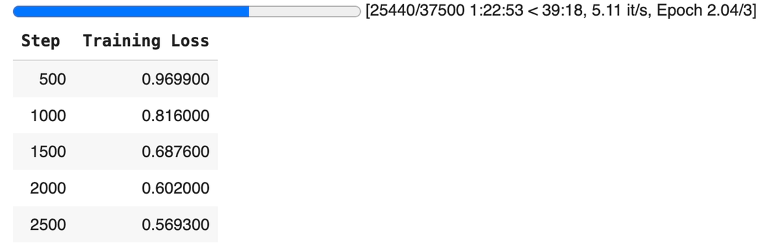
Figure 2: Google Colab terminal output from the training process using sentence-transformers.

Step refers to the current iteration of the training loop. It is an indicator of how many batches have been processed. If you see "Step 10", it means the trainer has processed 10 batches of data. Each step usually corresponds to one forward and backward pass through the model with one batch of data.

Training Loss is a measure of how well the model is performing on the training data at each step. The loss function calculates the difference between the model's predictions and the actual target values. The objective of training is to minimize this loss.

As we can see, the training loss is decreasing as the training loops through higher iterations. This is a good sign!

Evaluating the Trained Model

After fine-tuning, we can evaluate the model using a TripletEvaluator to assess its performance on the test set. This will tell us how well our fine-tuning has done.

Let’s first evaluate our initial pre-trained model before any fine-tuning.


old_model = SentenceTransformer(
    "microsoft/mpnet-base",
)

test_evaluator = TripletEvaluator(
    anchors=test_dataset["anchor"],
    positives=test_dataset["positive"],
    negatives=test_dataset["negative"],
    name="all-nli-test",
)
test_evaluator(old_model)

Here, we define the default base model we had to begin with as old_model. We set up a test_evaluator which will assess the model’s performance on the test_dataset.

This will provide accuracy metrics for our model using different distance measures. If you’re unfamiliar with distance metrics, we cover them in this article.


{'all-nli-test_cosine_accuracy': 0.6594038432440611,
 'all-nli-test_dot_accuracy': 0.452262066878499,
 'all-nli-test_manhattan_accuracy': 0.7147828718414283,
 'all-nli-test_euclidean_accuracy': 0.6562263579966712,
 'all-nli-test_max_accuracy': 0.7147828718414283}

These are the outputs. The description provides us with information about the similarity metric. The value indicates that the model correctly identified the positive example over the negative example X% of the time using said similarity measure.

For example,


'all-nli-test_cosine_accuracy': 0.6594038432440611,

says that the model correctly identified the positive example over the negative example 65.94% of the time using cosine similarity.

These are average results; the similarity measures are generally quite low and are in need of improvement. Let’s see if our newly fine-tuned model improves these.

We set up an evaluator again but this time, on our fine-tuned model.


test_evaluator = TripletEvaluator(
    anchors=test_dataset["anchor"],
    positives=test_dataset["positive"],
    negatives=test_dataset["negative"],
    name="all-nli-test",
)
test_evaluator(model)

This returns the output:


{'all-nli-test_cosine_accuracy': 0.908760780753518,
 'all-nli-test_dot_accuracy': 0.08987743985474353,
 'all-nli-test_manhattan_accuracy': 0.9067937660765623,
 'all-nli-test_euclidean_accuracy': 0.9073990013617794,
 'all-nli-test_max_accuracy': 0.908760780753518}

We have high accuracy values for cosine, Manhattan, and Euclidean distances which indicate that our model performs well in distinguishing between positive and negative examples in the triplet evaluation. Awesome news! The low dot product accuracy, however, suggests that it is not an effective measure in this context and can be disregarded for evaluating our model.

We can see very clearly that our fine-tuning has significantly improved the overall performance of our model. Pretty cool!

Now, it’s not always the case that the more you fine-tune your model, the better it will become. There are several quantities that affect the overall performance of your model. Let’s take a look at what these are.

Quantities that Affect Performance

The following can affect the performance of your model during fine-tuning.

Data Quality and Quantity:
- Quality: The quality of the data used for fine-tuning is critical. Noisy, incomplete, or biased data can negatively impact model performance.
- Quantity: Having sufficient data is important. A larger, diverse dataset can help the model generalize better. Although this is typically more computational.
Learning Rate: The learning rate determines how quickly or slowly the model learns. Too high a learning rate can cause the model to converge too quickly to a suboptimal solution, while too low a learning rate can make the training process very slow or get stuck in local minima.
Batch Size: The size of the batches used for training can impact model performance. Larger batch sizes can lead to faster training but might require more computational resources. Smaller batch sizes might provide more stable training but can be slower.
Choice of Optimizer: Different optimizers (e.g., SGD, Adam, RMSprop) have different properties and can affect the convergence speed and final performance of the model.

There are so many other arguments that can affect the performance of your model when fine-tuning. We’ve used a generic example in this article but it’s worth noting that you can change these arguments to best suit your needs. This article on Hugging Face dives a bit deeper on further specifications.

3. Conclusion

In this article we have covered how you can fine-tune your own sentence transformer using Hugging Face’s sentence-transformer library. During this, we saw how implementing fine-tuning can result in significant improvements in the model’s performance.

We have now covered sentence transformers which allow for computers to understand words and sentences but what about images? Join us in the next article where we learn about Vision Transformers and how we can fine-tune those too!